线性回归 (Linear Regression)

线性回归（Linear Regression）是机器学习中最基础且广泛应用的算法之一。

线性回归 (Linear Regression) 是一种用于预测连续值的最基本的机器学习算法，它假设目标变量 y 和特征变量 x 之间存在线性关系，并试图找到一条最佳拟合直线来描述这种关系。

y = w * x + b

其中：

• y 是预测值

• x 是特征变量

• w 是权重 (斜率)

• b 是偏置 (截距)

线性回归的目标是找到最佳的 w 和 b，使得预测值 y 与真实值之间的误差最小。常用的误差函数是均方误差 (MSE)：

MSE = 1/n * Σ(y_i - y_pred_i)^2

其中：

• y_i 是实际值。
• y_pred_i 是预测值。
• n 是数据点的数量。

我们的目标是通过调整 w 和 b ，使得 MSE 最小化。

如何求解线性回归？

1、最小二乘法

最小二乘法是一种常用的求解线性回归的方法，它通过求解以下方程来找到最佳的 ( w ) 和 ( b )。

最小二乘法的目标是最小化残差平方和（RSS），其公式为：

$$\text{RSS}=\sum \mathrm{\_}{i=1}^n(y\mathrm{\_}i-\hat{y}\mathrm{\_}i{)}^2$$

其中：

• \( y_i \) 是实际值。
• \( \hat{y}_i \) 是预测值，由线性回归模型 \( \hat{y}_i = w x_i + b \) 计算得到。

通过最小化 RSS，可以得到以下正规方程：

$$\{\begin{array}{l}w\sum \mathrm{\_}{i=1}^{n}x\mathrm{\_}{i}^2+b\sum \mathrm{\_}{i=1}^{n}x\mathrm{\_}i=\sum \mathrm{\_}{i=1}^{n}x\mathrm{\_}iy\mathrm{\_}i\\ w\sum \mathrm{\_}{i=1}^{n}x\mathrm{\_}i+bn=\sum \mathrm{\_}{i=1}^{n}y\mathrm{\_}i\end{array}$$

矩阵形式

将正规方程写成矩阵形式：

$$\left[\begin{array}{cc}\sum \mathrm{\_}{i=1}^{n}x\mathrm{\_}{i}^2& \sum \mathrm{\_}{i=1}^{n}x\mathrm{\_}i\\ \sum \mathrm{\_}{i=1}^{n}x\mathrm{\_}i& n\end{array}\right]\left[\begin{array}{c}w\\ b\end{array}\right]=\left[\begin{array}{c}\sum \mathrm{\_}{i=1}^{n}x\mathrm{\_}iy\mathrm{\_}i\\ \sum \mathrm{\_}{i=1}^{n}y\mathrm{\_}i\end{array}\right]$$

求解方法

通过求解上述矩阵方程，可以得到最佳的 \( w \) 和 \( b \)：

$$\left[\begin{array}{c}w\\ b\end{array}\right]={\left[\begin{array}{cc}\sum \mathrm{\_}{i=1}^{n}x\mathrm{\_}{i}^2& \sum \mathrm{\_}{i=1}^{n}x\mathrm{\_}i\\ \sum \mathrm{\_}{i=1}^{n}x\mathrm{\_}i& n\end{array}\right]}^{-1}\left[\begin{array}{c}\sum \mathrm{\_}{i=1}^{n}x\mathrm{\_}iy\mathrm{\_}i\\ \sum \mathrm{\_}{i=1}^{n}y\mathrm{\_}i\end{array}\right]$$

2、梯度下降法

梯度下降法的目标是最小化损失函数 \( J(w, b) \) 。对于线性回归问题，通常使用均方误差（MSE）作为损失函数：

$$J(w,b)=\frac{1}{2m}\sum \mathrm{\_}{i=1}^m(y\mathrm{\_}i-\hat{y}\mathrm{\_}i{)}^2$$

其中：

• \( m \) 是样本数量。
• \( y_i \) 是实际值。
• \( \hat{y}_i \) 是预测值，由线性回归模型 \( \hat{y}_i = w x_i + b \) 计算得到。

梯度是损失函数对参数的偏导数，表示损失函数在参数空间中的变化方向。对于线性回归，梯度计算如下：

$$\frac{\partial J}{\partial w}=-\frac{1}{m}\sum \mathrm{\_}{i=1}^{m}x\mathrm{\_}i(y\mathrm{\_}i-\hat{y}\mathrm{\_}i)$$$$\frac{\partial J}{\partial b}=-\frac{1}{m}\sum \mathrm{\_}{i=1}^m(y\mathrm{\_}i-\hat{y}\mathrm{\_}i)$$

参数更新规则

梯度下降法通过以下规则更新参数 \( w \) 和 \( b \)：

$$w:=w-\alpha \frac{\partial J}{\partial w}$$$$b:=b-\alpha \frac{\partial J}{\partial b}$$

其中：

• \( \alpha \) 是学习率（learning rate），控制每次更新的步长。

梯度下降法的步骤

1. 初始化参数：初始化 \( w \) 和 \( b \) 的值（通常设为 0 或随机值）。
2. 计算损失函数：计算当前参数下的损失函数值 \( J(w, b) \)。
3. 计算梯度：计算损失函数对 \( w \) 和 \( b \) 的偏导数。
4. 更新参数：根据梯度更新 \( w \) 和 \( b \)。
5. 重复迭代：重复步骤 2 到 4，直到损失函数收敛或达到最大迭代次数。

使用 Python 实现线性回归

下面我们通过一个简单的例子来演示如何使用 Python 实现线性回归。

1、导入必要的库

实例

import numpy as np

import matplotlib.pyplot as plt

from sklearn.linear_model import LinearRegression

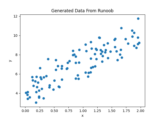
2、生成模拟数据

实例

import numpy as np

import matplotlib.pyplot as plt

from sklearn.linear_model import LinearRegression

# 生成一些随机数据

np.random.seed(0)

x = 2 * np.random.rand(100, 1)

y = 4 + 3 * x + np.random.randn(100, 1)

# 可视化数据

plt.scatter(x, y)

plt.xlabel('x')

plt.ylabel('y')

plt.title('Generated Data From Runoob')

plt.show()

显示如下所示：

3、使用 Scikit-learn 进行线性回归

实例

import numpy as np

import matplotlib.pyplot as plt

from sklearn.linear_model import LinearRegression

# 生成一些随机数据

np.random.seed(0)

x = 2 * np.random.rand(100, 1)

y = 4 + 3 * x + np.random.randn(100, 1)

# 创建线性回归模型

model = LinearRegression()

# 拟合模型

model.fit(x, y)

# 输出模型的参数

print(f"斜率 (w): {model.coef_[0][0]}")

print(f"截距 (b): {model.intercept_[0]}")

# 预测

y_pred = model.predict(x)

# 可视化拟合结果

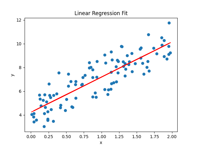
plt.scatter(x, y)

plt.plot(x, y_pred, color='red')

plt.xlabel('x')

plt.ylabel('y')

plt.title('Linear Regression Fit')

plt.show()

输出结果：

斜率 (w): 2.968467510701019
截距 (b): 4.222151077447231

显示如下所示：

我们可以使用 score() 方法来评估模型性能，返回 R^2 值。

实例

import numpy as np

from sklearn.linear_model import LinearRegression

# 生成一些随机数据

np.random.seed(0)

x = 2 * np.random.rand(100, 1)

y = 4 + 3 * x + np.random.randn(100, 1)

# 创建线性回归模型

model = LinearRegression()

# 拟合模型

model.fit(x, y)

# 计算模型得分

score = model.score(x, y)

print("模型得分:", score)

输出结果为：

模型得分: 0.7469629925504755

4、手动实现梯度下降法

实例

import numpy as np

import matplotlib.pyplot as plt

from sklearn.linear_model import LinearRegression

# 生成一些随机数据

np.random.seed(0)

x = 2 * np.random.rand(100, 1)

y = 4 + 3 * x + np.random.randn(100, 1)

# 初始化参数

w = 0

b = 0

learning_rate = 0.1

n_iterations = 1000

# 梯度下降

for i in range(n_iterations):

    y_pred = w * x + b

    dw = -(2/len(x)) * np.sum(x * (y - y_pred))

    db = -(2/len(x)) * np.sum(y - y_pred)

    w = w - learning_rate * dw

    b = b - learning_rate * db

# 输出最终参数

print(f"手动实现的斜率 (w): {w}")

print(f"手动实现的截距 (b): {b}")

# 可视化手动实现的拟合结果

y_pred_manual = w * x + b

plt.scatter(x, y)

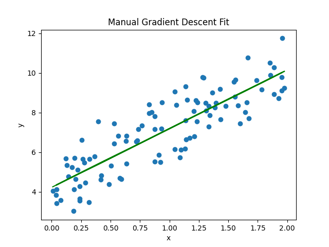
plt.plot(x, y_pred_manual, color='green')

plt.xlabel('x')

plt.ylabel('y')

plt.title('Manual Gradient Descent Fit')

plt.show()

输出结果：

手动实现的斜率 (w): 2.968467510701028
手动实现的截距 (b): 4.222151077447219

显示如下所示：

AI 思考中...

机器学习算法

逻辑回归（Logistic Regression）